User manual

1. Running the program

To run the program, you have to have Java 1.8+ installed on your computer (chances are you already have it). If not, see here: http://www.java.com/en/download/help/index_installing.xml

The program can be started either (depending on the OS) by:

 * from the GUI: double-clicking the g.jar 
 * from the console: when positioned in the program folder, type: "java -jar GisaxStudio.jar"

The latter will print the potential errors into the console, which helps in error reporting/debugging

1. Setup new experiment

Upon start, the program will report that there are no "experiments" in the database.

• • Note: the program relies on the database to store/retrieve all data related to the experiments EXCEPT IMAGES which are kept in the file system.**

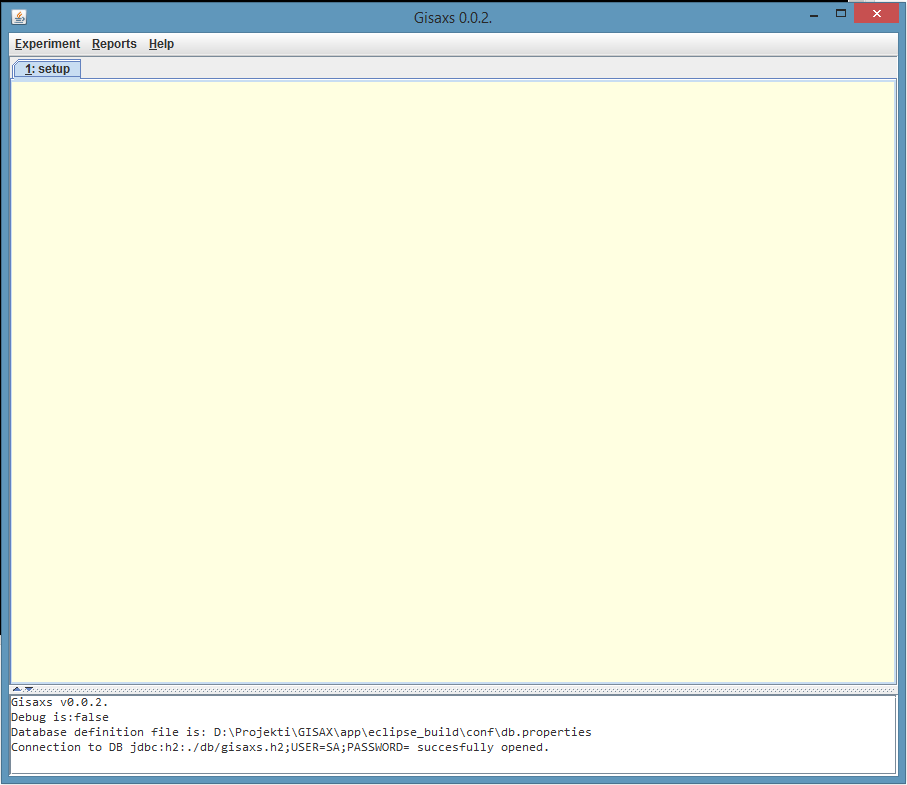
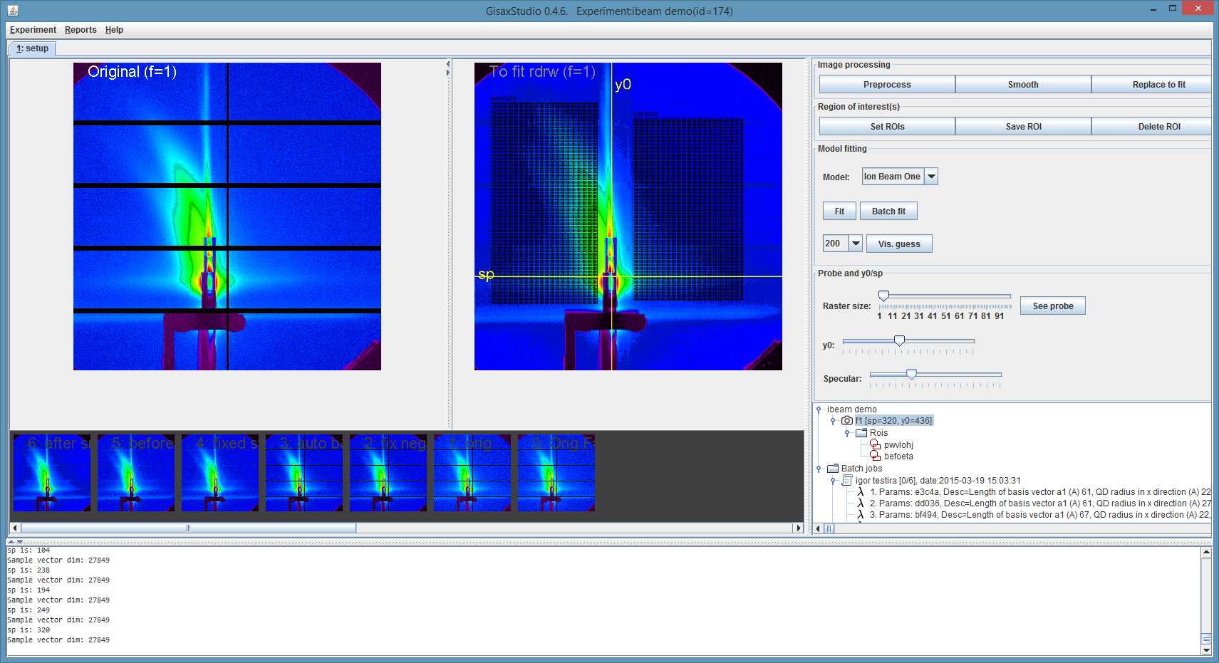
Data processing is logically organized into "experiments" - experiment being a way of grouping a number of images (N>=1) to be fitted. An experiment can consist of 1+ frames (images) and there can be any number of experiments in the database. It is up to the user to structure (group) his/hers data into experiments. Initial screen:

Choose: Experiment->New experiment

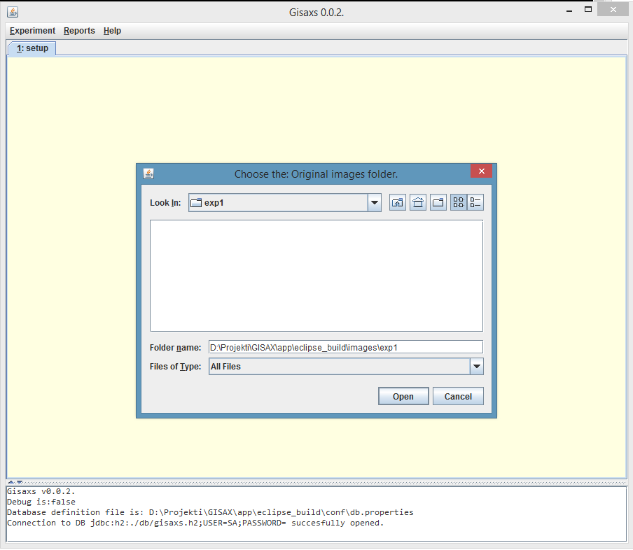
Select the folder where you experiment's images (to fit) reside. There are already two test images provided with the download in the /images/exp1 folder. It is recommended to user relative paths, that is - to store images in the provided "images" folder, using subfolder named after the experiment. This way the program (and images) can be easily copies from one computer to another without additional configuration. Contrary, if you use absolute paths and point to e.g. c:\temp\images, that folder might not exist on another computer.

Here, images/exp1 is chosen:

Name the experiment:

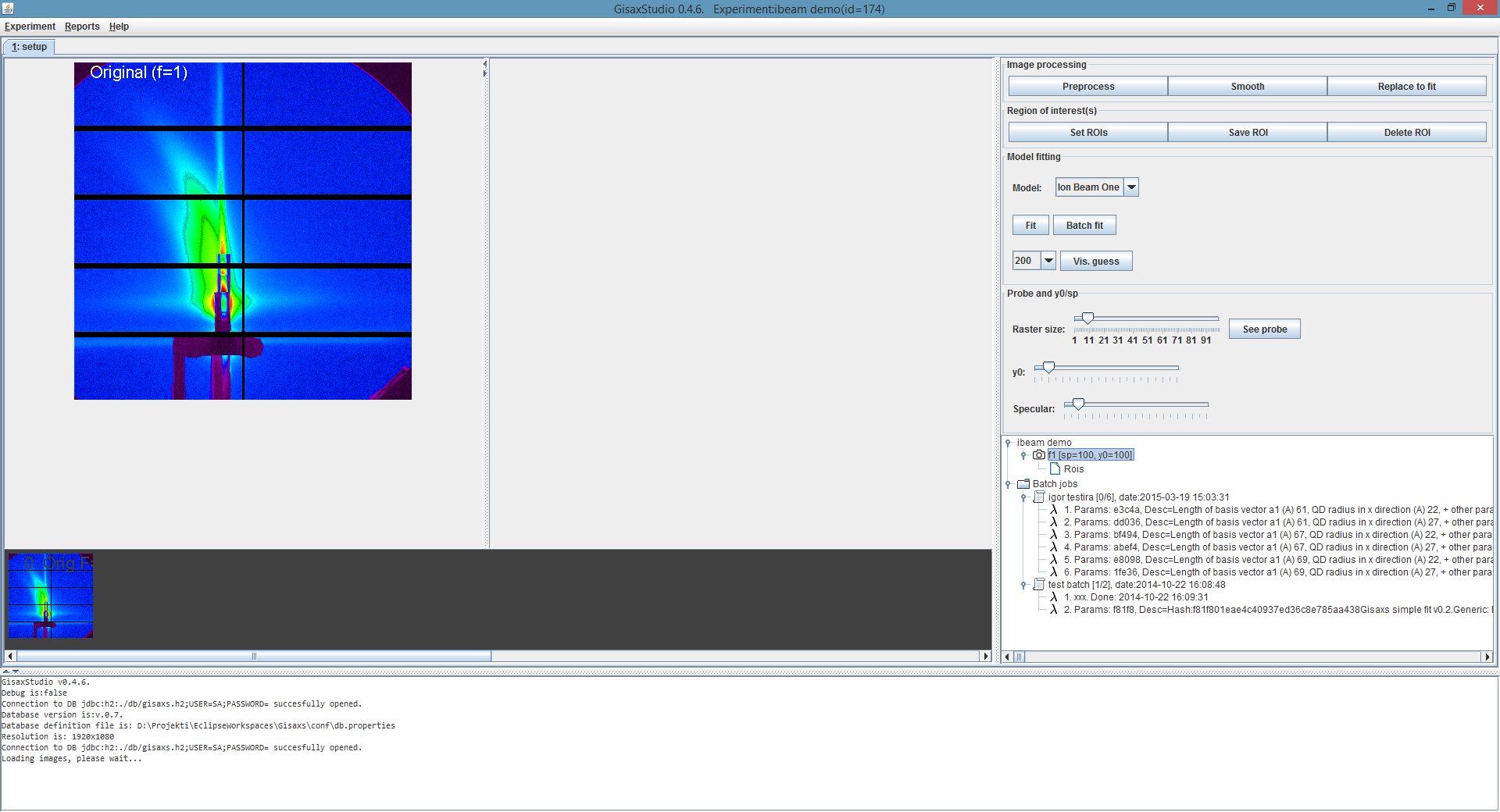
Depending on the number of tif images found there, the program will setup "frames". There has to be at least one tif image in the assigned folder. In this example, there are two images in the /images/exp1 folder and so we have:

2. Layout

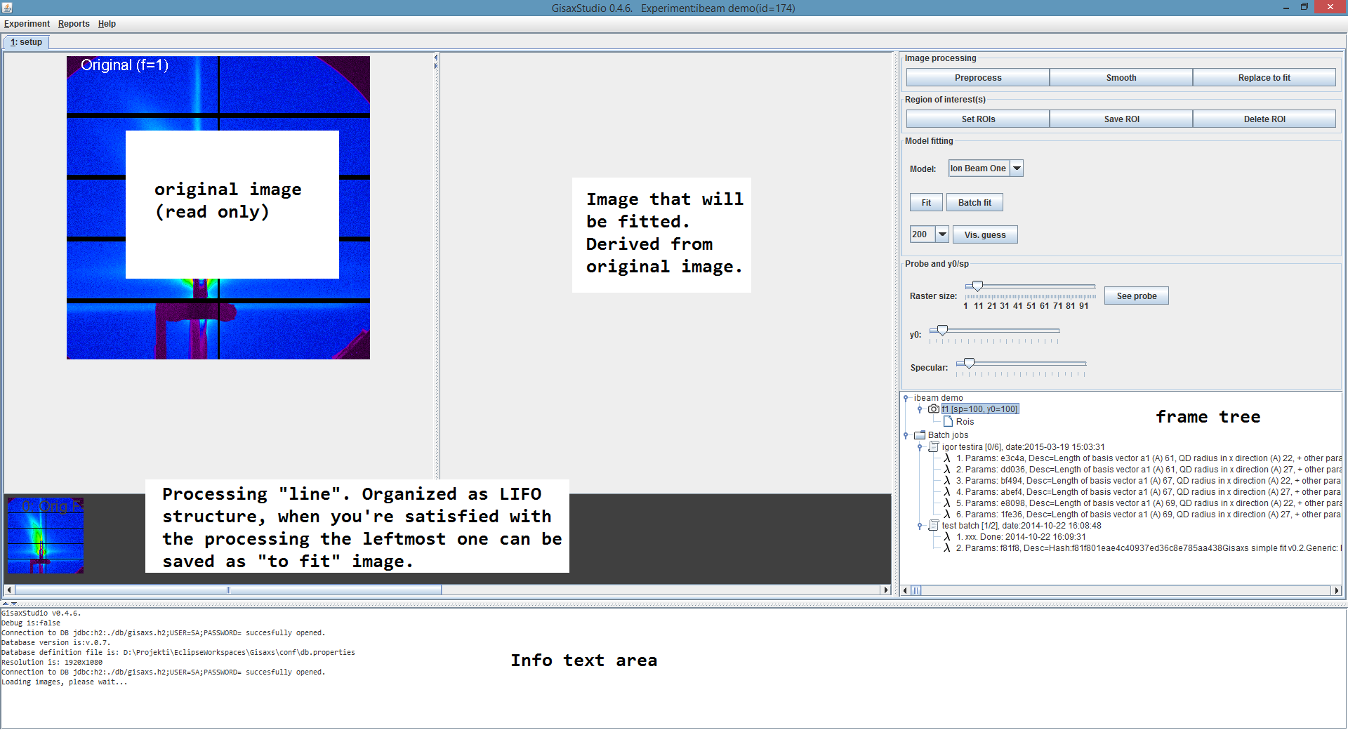
Program layout is organized as shown here:

3. Preprocess the image

It is intended for image processing tasks (e.g. image resize) to take place outside of the program, using one of many image processing tools (e.g. ImageJ). However, some rudimentary image processing operations are built into the program, namely "Preprocess" which consists of:

 1. Fixing negative values ( by setting them to zero)
 2. Auto brightness & contrast
 3. Fixing "dark stripes sometimes produced by detector" by interpolation

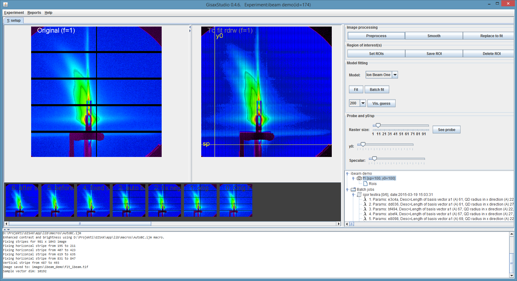
So, in our test experiment, **click "Smooth"** until you're satisfied with the image. Then, assign the leftmost image to be the "fit image" by clicking on "-> to fit" button:

4.1. Sampling areas (ROIs)

Now that we have prepared the image, we need to define the sampling areas. If not, the whole image will be sampled.

• • Click on the "Set ROIs"** button. A new image will pop-up, along with the ImageJ application.

Use ImageJ's selection tools to assign the sampling areas by: (a) selecting the area (b) clicking the Save ROI button

==>

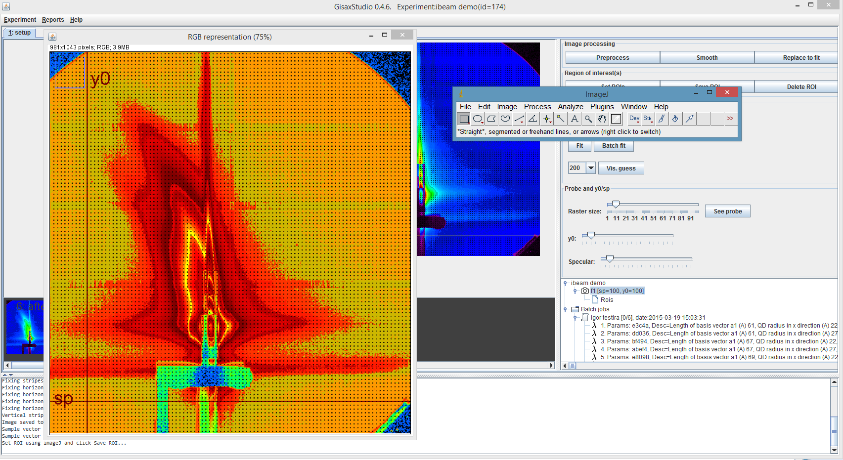
If you assign multiple ROIs (selections) a UNION of those areas will be used. Each ROI is given a generated name, and you can delete it afterwards (it is visible in the Frame tree). You can also add more ROIs later. Close manually ImageJ and SetRoi window once you're done.

4.2. Raster size/specular/y0

Adjust the raster size, specular and y0 using provided sliders. Fit image reflects the assigned values.

5. Running single fit

Select the frame you want to fit in the frame tree and click "Fit" button.

A dialog with additional model parameters is presented. Adjust the values if needed and click "Run". Parameter values are automatically stored in the database (if such combination doesn't already exist).

After a 10-20 seconds, a new tab will appear in which all available fitting/optimizing algorithms will be started (in separate threads):

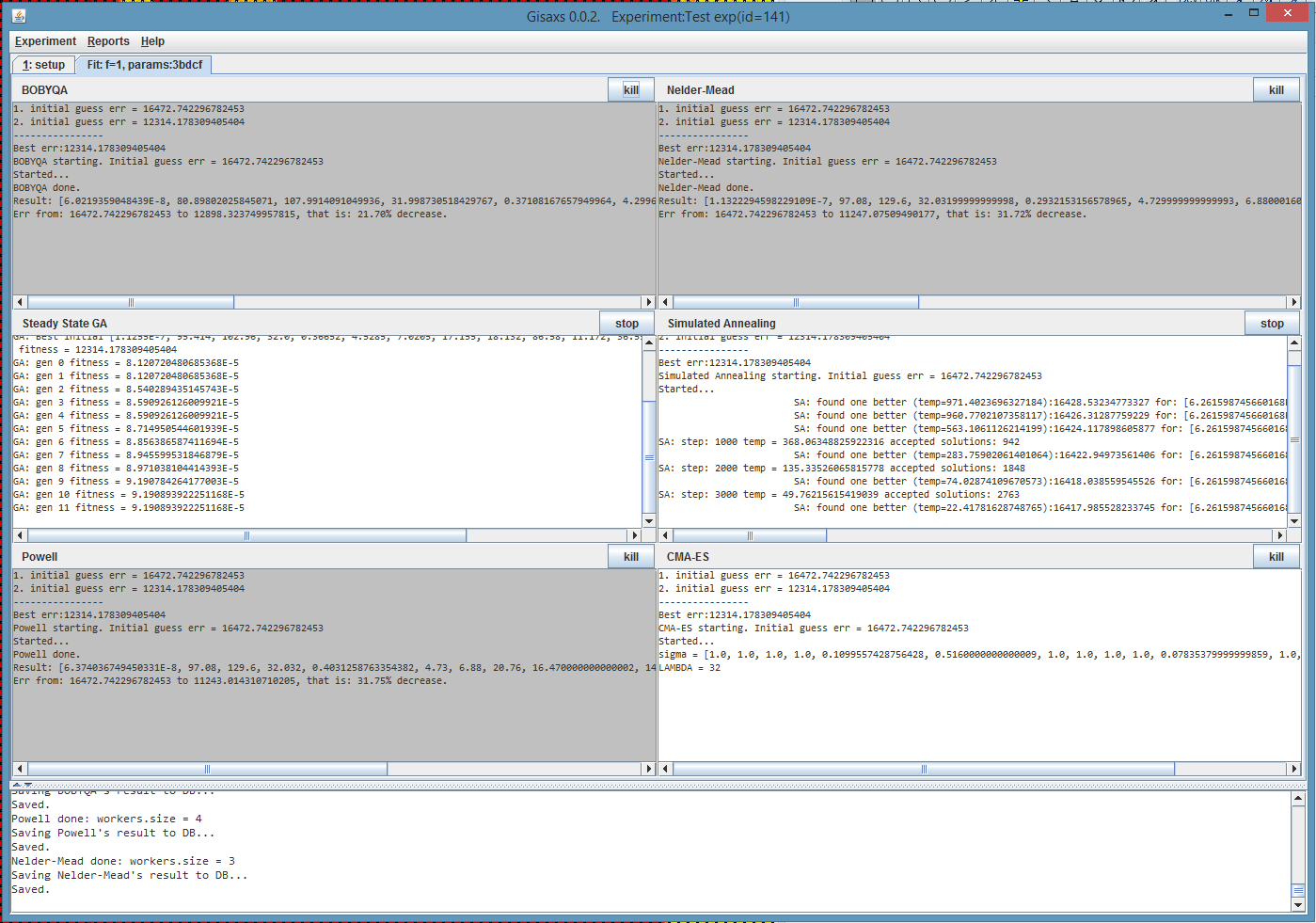
When they are done, the results will be stored in the database (and visible in the Frame tree, under the corresponding parameter node).

Note that you can stop/kill some algorithms if you wish, the difference being:

 * stop - gracefully stops the algorithm, and the results obtained so far are stored in the DB
 * kill - ungracefully stops the algorithm, no results from that algorithm are stored

6. Running batch fit

To run a batch fit, one must first define a number of parameters that will be used. So (a) the parameters have to be defined, stored in the DB, and then (b) one can run a batch on those params.

6.1. Batch parameters definition

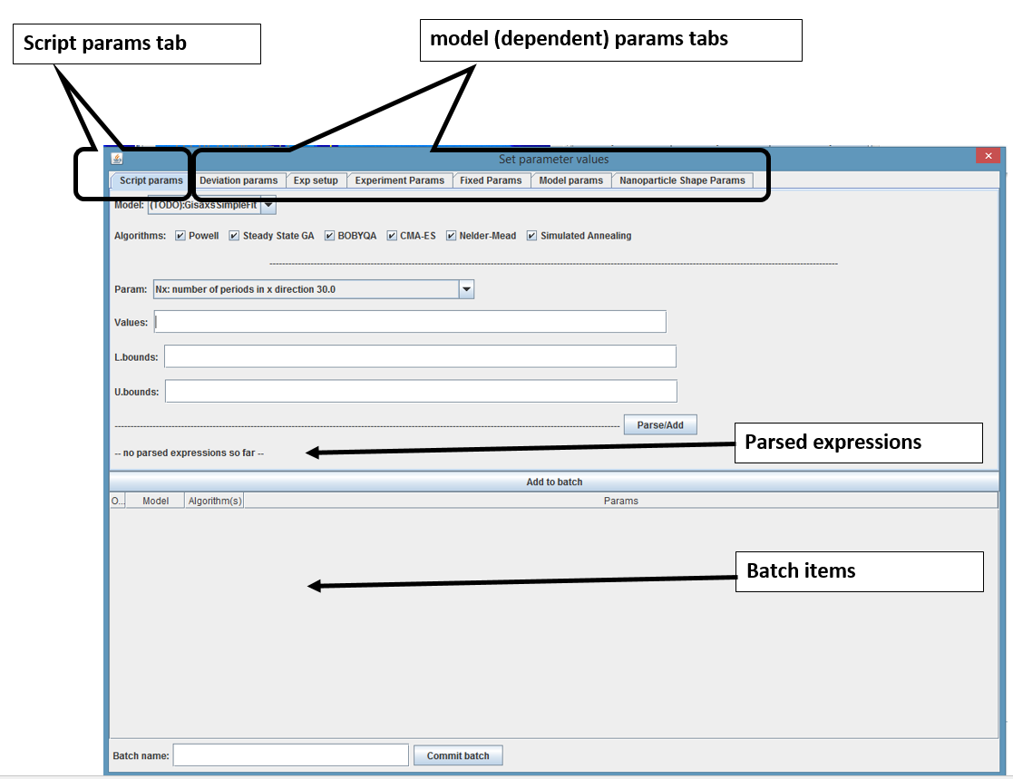
Select the frame you want to fit in the frame tree **and click "Batch Fit" button.** The same dialog as in single fit appears, but with additional tab that allows for programmatic parameter variations to be defined.

There are two approaches to parameters definition:

 * manual: vary parameters by hand and add them to the batch items set.
 * using script params tab: assign expressions for each parameter you want to vary

6.1.1. Manual definition

Set model parameters using model dependent tabs and click "add to batch". Repeat as many times as needed. Note that manual definition can be combined with the "script approach", for instance you can define e.g. 3 batch items manually and then continue to add another N items using the script tab:

6.1.2. Using script tab

The upper part of the script tab (model & algorithms) actually pertains to both approaches - it is used to:

 * select the model (only one for the time being). Changing model causes the model dependent tabs to reload (TODO).
 * select the algorithms that will be used (regardless of what approach was used).

The lower part allows to select any of the current model parameters and to set **the list of values** that will be used/varied (iterated). Upper and lower bounds can also be assigned, but in that case the bounds list cardinality must be equal to the values list cardinality.

 E.g. 
 if we want to vary param A using values: 1, 2 and 3
 we can also assign upper and lower bounds, but there has to be three of each.

• • The list of values** (expressions) can be assigned in two ways:

 * manual lists, examples: 
   * "1, 5,   7"
   * "(1, 2),  (3, 4)"    -> those are complex numbers 1+2i, 3+4j

 * for expression (that evaluates to a list):
   * "for(1; 10; 3)"   -> evaluates to "1, 4, 7, 10"
   * "for( (1, 1); (3, 3); (1, 1) )"   -> evaluates to "(1, 1), (2, 2), (3, 3)", when using complex numbers abs is used to evaluate the middle <= expression 

When you define the values (and potentially the corresponding bound expressions), click the "Parse/Add" button to see whether the program accepts the syntax and successfully parses the expression into list. You can define a number of such lists using different model parameters, and finally, when you're satisfied click "Add to batch" so that the batch items are generated and added to the list. If there are more than one lists, the program will generate a Cartesian product of those lists, while preserving the order.

 For instance, let say you've defined four lists (for params A, B, C and D):
 [1, 2, 3]
 ["A", "B"]
 ["x", "y"]
 [0., 3.14, 2.71]
 the program will generate 36 = 3 * 2 * 2 * 3 items:
 0. -->  1 A x 0.0
 1. -->  1 A x 3.14
 2. -->  1 A x 2.71
 3. -->  1 A y 0.0
 4. -->  1 A y 3.14
 5. -->  1 A y 2.71
 6. -->  1 B x 0.0
 7. -->  1 B x 3.14
 8. -->  1 B x 2.71
 9. -->  1 B y 0.0
 10. -->  1 B y 3.14
 11. -->  1 B y 2.71
 12. -->  2 A x 0.0
 13. -->  2 A x 3.14
 14. -->  2 A x 2.71
 15. -->  2 A y 0.0
 16. -->  2 A y 3.14
 17. -->  2 A y 2.71
 18. -->  2 B x 0.0
 19. -->  2 B x 3.14
 20. -->  2 B x 2.71
 21. -->  2 B y 0.0
 22. -->  2 B y 3.14
 23. -->  2 B y 2.71
 24. -->  3 A x 0.0
 25. -->  3 A x 3.14
 26. -->  3 A x 2.71
 27. -->  3 A y 0.0
 28. -->  3 A y 3.14
 29. -->  3 A y 2.71
 30. -->  3 B x 0.0
 31. -->  3 B x 3.14
 32. -->  3 B x 2.71
 33. -->  3 B y 0.0
 34. -->  3 B y 3.14
 35. -->  3 B y 2.71

You can also delete some of the generated items in the batch items list by double-clicking the item. So, for instance, you can define three items manually, then generate 36 more items, and then delete any number of items from the overall (3+36) list.

When you're done revising the items, you store them in the database by **giving a batch name** and clicking on the **commit batch** button.

Batch is then stored in the database and ready to be run:

6.1. Batch execution

All stored batch jobs appear in the Frame tree, under the "Batch jobs" node. To run the batch, select it (click on it), then right-click it and select "Run batch".

The program behaves as follows:

 repeat-until-there-are-unfinished-batch-items:
 |- load the first batch item (params) from list that has not been executed yet
 |- execute the batch item (fit)
 |- store the results to the database

Note that **the batch execution can be interrupted at any time and resumed afterwards!**

 For instance, let's say we run a 40 items batch.
 The program progresses to the e.g. 20th item and then the computer powers off (or a user simply kills the program).
 19 items have been executed and their results stored in the DB.
 20-th item was interrupted and those results are "lost".
 However, when the same batch is run afterwards, it will simply resume from the 20-th item and finish the whole batch.